Exploratory graphics
Data visualization
First of all, the LiDAR subsets were clipped from Stereocarto LiDAR data using the shapefile of selected 27 plots (45m * 45m). Then, visualize them in 3D and color them according to the canopy height (Figure 7). The LiDAR data derived two forest structure parameters, i.e., canopy height and leaf are density (LAD).

Figure 7. LiDAR data 3D visualization for 27 plots. The resolution is compressed due to the limitation of Weebly.
|
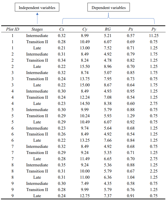
Table 2. Metrics derived from Leaf Area Density profile for 27 plots. Different successional stages will be set as independent variables, and metrics will be set as dependent variables in the subsequent analysis of variance (ANOVA).
|
Generation of Leaf Area Density (LAD) profiles
As mentioned above, the line chart can be plotted using leaf area density and canopy height derived from LiDAR data. This is actually a vertical leaf area density profile for each plot. According to corresponding successional stages, 27 LAD profiles were grouped into three groups: Intermediate, Transition II, and Late (Figure 8). The average of profiles within each group was calculated and plotted as a red line to help visualize the difference better.

Figure 8. The vertical Leaf Area Density (LAD) profile of 27 plots for the Intermediate (a), Transition II (b), and Late successional stage (c). The solid red line in each subfigure is the average for the corresponding nine waveforms.
Calculation of metrics
Five metrics were calculated for each profile based on the derived leaf area density profile from LiDAR data (Figure 8 & Table 2). In the case of the LAD profile (Figure 5 & Figure 8), Cx can be calculated as the mean leaf area density (m2/m3); Cy can be calculated as the mean canopy height (m); RG can be calculated by the formula (Figure 6); Px refers to the x coordinate of the maximum waveform amplitude (m2/m3); Py refers to the y coordinate of the maximum waveform amplitude (m). Based on this, some basic statistics, such as mean and standard deviation, could be calculated. Furthermore, analysis of variance (ANOVA) and pair comparison is expected to check if different successional stages have significant differences for several metrics.
