Results
|
The mean value and standard deviation of each metric for different successional stages are shown in Table 3. The intermediate successional plots have a higher mean value of Cx (0.31) than transition II (0.28) and late plots (0.25). In contrast, the mean value of Cy and RG increases with the successional gradient: from 8.69 to 10.30 (the intermediate stage to transition II) to 13.00 (transition II to the late stage) and from 5.13 to 5.96 (the intermediate stage to transition II) to 7.52 (transition II to the late stage), respectively. However, the higher standard deviation compared to the intermediate stage shows a noticeable fluctuation in Cy and RG of transition II and the late stage. The results also suggest an increase in the mean value of Px with the successional gradient; besides, transition II shows a higher standard deviation in Px.
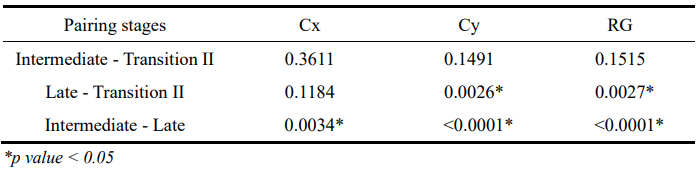
ANOVA results show that different successional stages have significant differences in three shape-based metrics: Cx, Cy, and RG (Table 3). Pair comparison results are shown in Table 4: for these three significant metrics, all p values are larger than 0.05 (Intermediate-Transition II). Late-Transition II shows significant differences in Cy and RG, and Intermediate-late shows significant differences in all three shape-based metrics. However, pair comparison cannot prove that there is no difference in metrics between intermediate and transition II, although p values are larger than 0.05. Instead, the difference between intermediate and transition II can be seen in LiDAR data visualization (Figure 7), LAD profiles (Figure 8), and violin plots (Figure 9). |
Table 3. Mean (±SD) and ANOVA p value of metrics derived from 27 plots over two successional stages and one transition at the SRNP-EMSS, Guanacaste, Costa Rica.
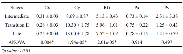
Table 4. Pair comparison results for significant metrics (Cx, Cy, and RG) with successional stages.
|
Discussion

Figure 9. Violin plots for the LiDAR metrics (Cx, Cy, Px and Py) distribution from 27 plots at the SRNP-EMSS, Guanacaste, Costa Rica. (a) The change of Cx with successional stages. (b) The change of Cy with successional stages. (c) The change of Px with successional stages. (d) The change of Py with successional stages.
|
Cx (the mean of LAD) is decreasing (Figure 9a & Table 3) along the successional path (Intermediate–Transition II–Late); this can be explained as the intermediate stage is infested by lianas most seriously, and lianas abundance decreases from the intermediate to the late stage (Sanchez-Azofeifa et al. 2017). Thus, most lianas are put on leaves, leading to overestimating LAD in the intermediate stage. Meanwhile, canopy gaps decrease from the intermediate to the late stage, leading to the lack of sunlight. As a result, more lianas are killed in transition II and the late stage.
Cy (the mean of canopy height) shows an increasing trend with successional stages (Figure 9b & Table 3). This is easy to explain because trees are growing. Those mature trees usually tend to be higher than young trees. In contrast, no such significant differences exist in Px and Py with successional stages (Figure 9c, Figure 9d and Table 3). The reasonable explanation for this is that almost all intermediate, transition II and late successional forest patches at the SRNP-EMSS are covered by dense shrubs, tall grasses, or short trees, which leads to the corresponding maximum peak occurring close to the ground of the vertical profile of all three successional stages. |
|
The larger RG reflected as an irregular waveform distribution in vertical profiles. Besides, the standard deviation also shows something: compared to the intermediate stage, RG shows a higher standard deviation in transition II and the late stage (Figure 10 & Table 3). These may be interpreted as resulting from heterogeneity in the forest: Transition II and the late stage create more heterogeneous space than the intermediate stage. In addition, unevenly aged trees and mixed species increase along Intermediate - Transition II - Late. The forest is becoming more dynamic, and the waveform variation within each stage tends to become irregular from Intermediate to Late.
The scatter plot links the RG to the LAD (Figure 10). There is a clear distinction between the intermediate and late stages. However, plots in transition II show a prominent transition feature, which spreads among the intermediate and late stages. We also can see that a few green triangles are much further away from others, which might be caused by the misclassification from the classification map of successional gradients (Figure 3b). But, this highlights the dynamic and uncertainty of transitions to some extent. |

Figure 10. A scatter plot of RG (the radius of gyration) versus LAD (leaf area density) from 27 plots distributed along the successional gradient (Intermediate, Transition II and Late) at the SRNP-EMSS, Guanacaste, Costa Rica.
|
Conclusion
This project characterized the forest structure of transitions using LiDAR data and derived metrics. My work highlights (1) transitional features (although they are subtle) are shown between intermediate and late successional stages, which means the succession is a continuous process and transitions work like a buffer in this process; (2) based on that, the existence of transitions in secondary succession is proven again; (3) shape-based metrics (Cx, Cy, and RG) can successfully capture the variability of the different waveform distribution, which is expected to change with the vertical structure. These findings support the previous work conducted by Li et al. (2017). Finally, carbon sequestration capacity and species composition changes are always research hot spots; the results of this project will provide an idea to study forest transitions in other aspects, such as biomass estimation, carbon sequestration capacity and species composition changes, in future work.
